2 The Data Science Life Cycle
This is the Open Access web version of Veridical Data Science. A print version of this book is published by MIT Press. This work and associated materials are subject to a Creative Commons CC-BY-NC-ND license.
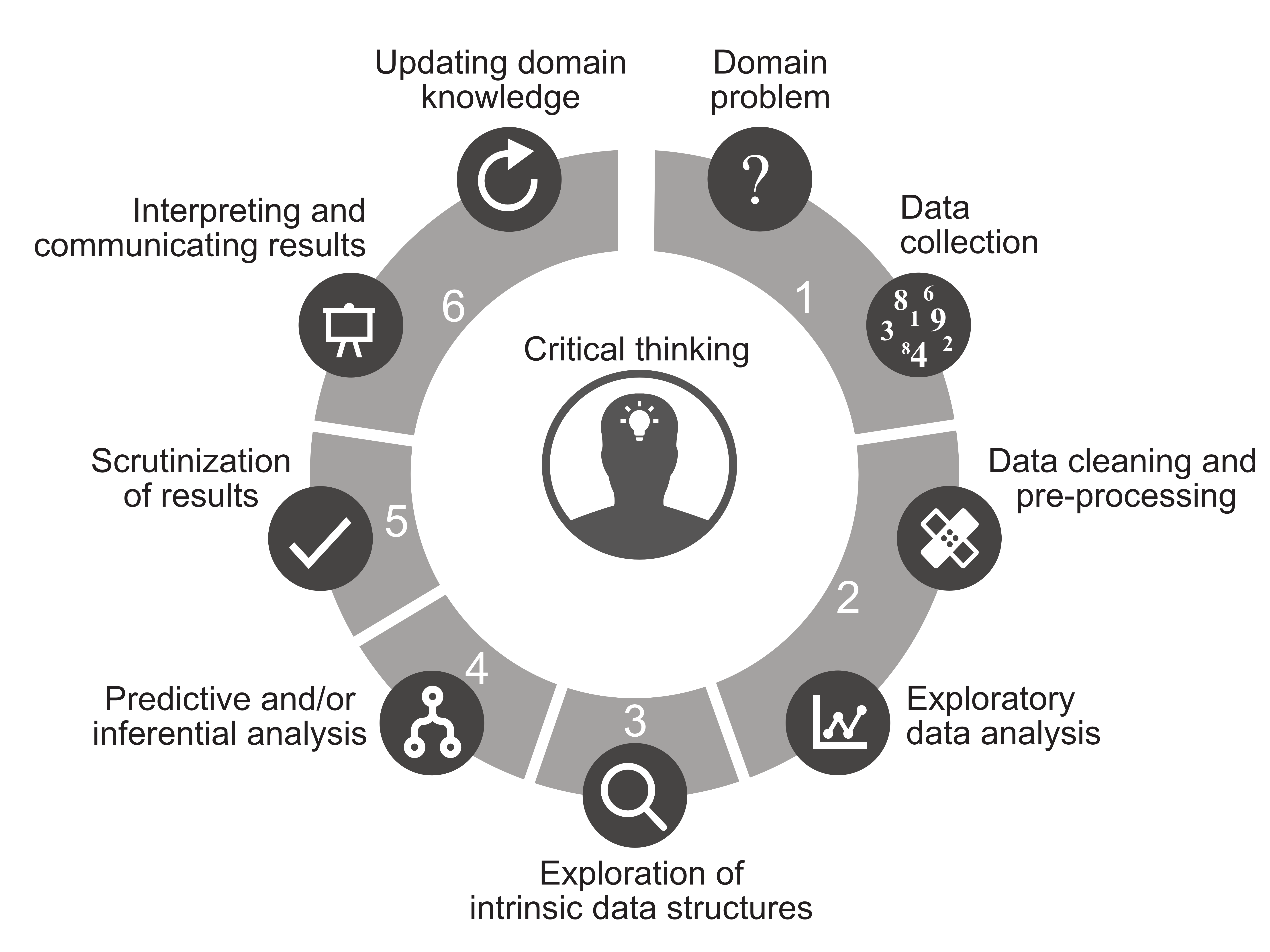
Every data science project progresses through some combination of the following stages of the data science life cycle (DSLC) (Figure fig-ds-cycle):
Domain problem formulation and data collection
Data cleaning, preprocessing, and exploratory data analysis
Exploration of intrinsic data structures (dimensionality reduction and clustering)
Predictive and/or inferential analysis
Evaluation of results
Communication of results
While almost every data science project will pass through stages 1–2 and 5–6, not every project will involve stages 3–4. Whether your project includes these stages will depend on the question that you are asking.
Although your project must pass through the first two stages of the DSLC before proceeding to the later stages, you will frequently find yourself returning to—and refining—these early stages as you progress. That is, the DSLC is not a strict linear process. In this chapter, we will provide a summary of each stage of the DSLC presented in Figure fig-ds-cycle, which will set the scene for the rest of this book. Part II of this book will focus on stages 2 and 3 of the DSLC, and part III will focus on predictive analysis—that is, stage 4 of the DSLC (note that we do not cover inferential analysis in this book). The final stages of evaluating and communicating results will be interspersed throughout the book.
2.1 Data Terminology
So far, we have only talked about “data” in the abstract. Before we introduce the stages of the DSLC, let’s look at an example of some actual data and introduce the data terminology that we will be using throughout this book. Table tbl-govt-spending presents a small dataset containing information on the annual US government spending and budgeting (in billions) for research and development (R&D), with explicit spending amounts provided for climate and energy.1
| Year | Budget | Total | Climate | Energy | Party |
|---|---|---|---|---|---|
| 2000 | 142,299 | 1,789,000 | 2,312 | 13,350 | Democrat |
| 2001 | 153,197 | 1,862,800 | 2,313 | 14,511 | Republican |
| 2002 | 170,354 | 2,010,900 | 2,195 | 14,718 | Republican |
| 2003 | 192,010 | 2,159,900 | 2,689 | 15,043 | Republican |
| 2004 | 199,104 | 2,292,800 | 2,484 | 15,343 | Republican |
| 2005 | 200,099 | 2,472,000 | 2,284 | 14,717 | Republican |
| 2006 | 199,429 | 2,655,000 | 2,004 | 14,194 | Republican |
| 2007 | 201,827 | 2,728,700 | 2,044 | 14,656 | Republican |
| 2008 | 200,857 | 2,982,500 | 2,069 | 15,298 | Republican |
| 2009 | 201,275 | 3,517,700 | 2,346 | 16,492 | Democrat |
| 2010 | 204,556 | 3,457,100 | 2,512 | 17,071 | Democrat |
| 2011 | 194,256 | 3,603,100 | 2,736 | 16,399 | Democrat |
| 2012 | 188,944 | 3,536,900 | 2,695 | 16,215 | Democrat |
| 2013 | 172,121 | 3,454,600 | 2,501 | 15,616 | Democrat |
| 2014 | 175,383 | 3,506,100 | 2,538 | 17,113 | Democrat |
| 2015 | 174,608 | 3,688,400 | 2,524 | 19,378 | Democrat |
| 2016 | 185,885 | 3,852,600 | 2,609 | 20,134 | Democrat |
| 2017 | 163,606 | 3,981,600 | 2,800 | 19,595 | Republican |
Each column of a data table (also referred to simply as the “data” or a “dataset”) corresponds to a different type of measurement and these are called the variables, features, attributes, or covariates of the data (in this book, we use these terms interchangeably to refer to the columns). Each variable in a dataset typically has one of the following types:
Numeric: A continuous value (e.g., spending amount), a duration (e.g., the number of seconds that a patient can balance on one foot, or the amount of time that a visitor spends on your website), a count (e.g., the number of visitors to your website in a prespecified period, the number of animals that are observed in a particular location), etc.
Categorical: A set of finite/fixed groups or categories with a predetermined set of options such as political party, hospital department, country, genre, etc.
Dates and times: Dates and times can come in many different formats, such as “01/01/2020 23:00:05” or “Jan 1 2020.”
Structured (short) text: Text with a prespecified structure or length, such as a person’s name, a mail address, an email address, etc.
Unstructured (long) text: A larger body of text that doesn’t have a predefined structure such as entries in pathology reports or doctor’s notes, movie reviews, tweets, posts on Reddit, etc.
The data in Table tbl-govt-spending contains numeric and categorical features (we are treating the “year” variable as a numeric feature, but it could be considered a date feature).
The dimension of the data refers to the number of variables (columns) that it contains (and sometimes also the number of rows that it contains). So “high-dimensional data” typically refers to data that has a lot of variables (typically more than 100, but there is no set cutoff after which data becomes “high-dimensional”). The government spending data in Table tbl-govt-spending is six-dimensional, which is not considered to be high-dimensional.
Each row corresponds to a particular observation, observational unit, data unit, or data point (we use these terms interchangeably). These are the entities for which the measurements are collected. Observational units are often countries or people, but in the case of Table tbl-govt-spending, the observational units are years. Observational units can also be a combination, such as countries and years (if measurements are taken for each country and each year). Each cell/entry in the table contains the value of a particular variable for an individual observational unit.
This format, in which the data is arranged into columns (features/variables) and rows (observational units), is called rectangular or tabular data. While some data types—such as text and images—might at first glance seem to be fundamentally nonrectangular, they can often be converted to rectangular formats to which the rectangular-data-based techniques and approaches that you will find in this book can be applied.
The rest of this chapter summarizes each of the six stages of the DSLC.
2.2 DSLC Stage 1: Problem Formulation and Data Collection
2.2.1 Formulating a Question
The first stage of the DSLC involves collaborating with domain experts to reformulate a domain question into one that can be answered using available data. This might seem straightforward, but it is very common for the initial domain question to be unintentionally vague or unanswerable. The key is to narrow down the overall goal of the domain experts who are asking the question. What are they hoping to achieve with an answer to their question? Often the initial question that is being asked is not the right question to achieve their intended goal.
After nailing down the goals of the project, the next task is to identify what data is already available or can be collected to answer it. If the question cannot be answered using the available data, then it needs to be refined to something that can be.
Consider the example of a team of data scientists working at a hospital who have been tasked with helping to decrease the hospital’s rate of hospital-acquired infections (HAIs). The initial domain question posed to the data scientists was “Why have the rates of HAI increased in our hospital?” The first task is to identify the overall goal of the question. Are hospital management more interested in identifying which patients are at higher risk of an HAI so that they can try to prevent infections (e.g., by providing these patients with higher doses of antibiotics or speeding up discharge timelines), or are they more interested in identifying general hospital practices, such as surgical hygiene practices, that are leading to the overall increased rates of HAI so that they can implement a training program or intensify sanitation and sterilization protocols?
The data required to address the patient-focused goal and the data required for the practice-focused goal of the HAI project are quite different. If the goal is to identify patient infection risk factors, relevant historical data can be obtained directly from the hospital’s medical records, which will contain rich, detailed information about patients who have experienced HAIs in the past. On the other hand, if the goal is to learn whether the hospital’s surgical hygiene practices are related to the increased infection rates, this data may not be readily available and will need to be manually collected, such as by watching recorded video footage, physically observing surgeries, or conducting a survey. Learning about what data is available may shift the goals of the project. Since historical patient record data is much easier to obtain than surgery practice data, this may explicitly shift the focus of the project to identifying patient HAI risk factors rather than uncovering poor hygiene practices. Expect your initial question to be continually refined as you learn more about the specific data that is available, and about what kinds of answers might be useful.
Effective communication and collaboration with domain experts is a vital component of real-world research projects. However, for the data science projects discussed in this book, we face a challenge: the projects in this book each rely on publicly available data, and unfortunately, we do not have direct access to relevant domain collaborators. Ideally, we would have showcased real examples from our own collaborative research projects throughout this book. However, the majority of our collaborative projects are centered around solving real-world domain problems in the fields of medicine and healthcare. Given the sensitive nature of the data involved, sharing this data publicly would violate privacy concerns and ethical guidelines.
While not having direct access to domain experts limits our ability to gain deeper insights into specific industries, we do our best to learn about the domain for each project by reading scientific literature so that the projects that we present within this book still provide valuable opportunities for showcasing the various data science techniques and approaches in the context of a plausible domain problem.
2.2.2 Data Collection
While some projects will use existing data (whether from public repositories, internal company databases, historical electronic medical records, or past experiments), other projects will involve collecting new data. Whenever possible, data scientists should be involved in designing the data collection protocol and collecting the data itself. It is often the case that when data is collected without involving the people who will analyze it, the resulting data ends up being poorly suited to answering the questions being posed. While we do not explicitly cover experimental design and data collection protocols in this book, some classic references include “Statistics for Experimenters: Design, Innovation, and Discovery” (Box, Hunter, and Hunter 2005) and “Design and Analysis of Experiments with R” (Lawson 2014).
When using existing data that has already been collected, ideally, you will be working with live data that is kept up to date (e.g., is corrected when errors are identified and maintained by a human), and for which additional background information can be obtained (Gelman 2009). It is important to develop a detailed understanding of how the data was collected and what the values within it mean, so being in communication with the people who collected the data (or at least who know more about it than you) is very helpful. When relevant and feasible, it can be very helpful to physically visit the site of data collection to learn about the instruments and procedures used to collect the data that you are working with.
In contrast, data that was collected in the past and is now stagnant (e.g., it lives online in a public data repository that is not maintained) and for which no additional relevant information can be obtained, is considered dead data (Gelman 2009). When working with dead data, you have no way of verifying the assumptions that you make, making it difficult to ensure that the data is being correctly interpreted. As a result, the data-driven findings that you obtain from it may be less trustworthy.
Each project that we introduce in this book involves publicly available data that has already been collected. Some of the projects will involve live data (such as the organ donations data from the World Health Organization and the US Department of Agriculture’s food nutrition data, both of which were collected by reputable government organizations and are continually updated), and others will involve dead data (such as the Ames house price data and the online shopping e-commerce data, both of which were collected as a snapshot of data from a data source that does not keep the data updated and about which we can obtain substantially less information). However, in all cases, we have done our best to learn about the data collection mechanisms and obtain relevant data documentation.
Recall that real data almost never perfectly reflects reality, but knowing how a dataset was collected can give some sense of how the data is related to reality. At minimum, every dataset that you use should be accompanied by detailed data documentation (such as README files and codebooks) that describes how the data was collected and what measurements it contains. However, even good data documentation rarely paints the complete picture and is certainly no substitute for physical communication with a knowledgeable human.
2.2.3 Making a Plan for Evaluating Predictability
Before moving to the second stage of the DSLC, we recommend making a plan for evaluating the predictability of your eventual results. If you can collect additional data (which resembles the future data to which you will be applying your results or algorithms), then you should either collect it now or make a plan for collecting it later. If not, you may need to split your existing data into a training set and validation set (and a test set, if relevant), using a splitting technique that best reflects the relationship between your current data and the future data to which you will be applying your results (see sec-train-val-test in sec-veridical-ds).
2.3 DSLC Stage 2: Data Cleaning and Exploratory Data Analysis
2.3.1 Data Cleaning
Once you’ve settled on a question and have collected some relevant data, it is time to clean your data. A clean dataset is one that is tidy, appropriately formatted, and has unambiguous entries. The initial data cleaning stage is spent identifying issues with the data (such as strange formatting and invalid values) and modifying it so that its values are valid and it is formatted in a computational- and human-friendly way. Data cleaning is an incredibly important stage of the DSLC because it not only helps ensure that your data is being correctly interpreted by your computer, but it also helps you to develop a more detailed understanding of the information that the data contains as well as its limitations.
The goal of data cleaning is to create a version of your data that is maximally reflective of reality and will be correctly interpreted by your computer. Computers are machines of logic. While they can do complex mathematical computations in the blink of an eye, computers do not automatically know that humidity measurements should always fall between 0 and 100, nor do they know that the word “high” represents a larger magnitude than the word “low.” Your computer doesn’t realize that the first two columns in your data contain different versions of the same information, nor can it tell that the information reported in the “score” column should be interpreted as ordered numeric (rather than as unordered categorical) values.
To ensure that your computer is faithfully using the information contained in your data, you will need to modify your data (by writing code, not by modifying the raw data file itself) so that it is in line with what your computer “expects.” However, the process of data cleaning is necessarily subjective and involves making assumptions about the underlying real-world quantities being measured as well as judgment calls about which modifications are the most sensible (such as deciding whether to replace negative humidity measurements with zeros, with missing values, or whether to just leave them alone).
2.3.2 Preprocessing
Preprocessing refers to the process of modifying your cleaned data to fit the requirements of a specific algorithm that you want to apply. For example, if you will be using an algorithm that requires your variables to be on the same scale, you may need to transform them or if you will be using an algorithm that does not allow missing values, you may need to impute or remove them. It is during preprocessing that you may also want to conduct featurization, the process of defining new features/variables using the existing information in your data if you believe that these will be helpful for your analysis.
Just as with data cleaning, there is no single correct way to preprocess a dataset, and the procedure that you end up with typically involves a series of judgment calls, which should be documented in your code and documentation files.
While we find it helpful to treat data cleaning and preprocessing as distinct processes, the two processes are fairly similar and it is sometimes simpler to treat data cleaning and preprocessing as a single unified process.
Data cleaning and preprocessing are the focus of sec-cleaning, where we will provide some guidelines for identifying messiness in data, as well as a highly customizable data cleaning procedure that can be tailored to fit the unique cleaning and preprocessing needs of every individual dataset.
2.3.3 Exploratory Data Analysis
The next stage involves taking a deeper look at the data by creating informative tables, calculating informative summary statistics such as averages and medians, and producing informative visualizations. This stage typically has two sub-stages. The first sub-stage, exploratory data analysis (EDA), involves developing rough numeric and visual summaries of the data that will help you understand the data and the patterns that it contains, while the second sub-stage, explanatory data analysis, involves polishing the most informative exploratory tables and graphs to communicate them to external audiences.
An example of an exploratory data visualization based on the government spending data presented in Table tbl-govt-spending is the line plot shown in Figure fig-govt-spending-exploratory-explanatory(a), which was created very quickly in R to help us explore the annual US government’s R&D spending on climate and energy over time. Figure fig-govt-spending-exploratory-explanatory(b) shows a polished explanatory version of this visualization that we might show to an external audience (such as the public, or some government or business officials). Version (b) has been customized to tell a clearer story: energy spending tends to increase during Democratic presidencies, but climate spending is fairly stagnant, regardless of the political affiliation of the president. As an exercise at the end of this chapter, you will be asked to re-create these figures yourself.

sec-eda introduces a range of principles for creating compelling numeric and visual descriptions of your data.
2.3.4 Data Snooping and PCS
While exploring your data is an extremely important part of the DSLC, it is not without risk. Data snooping is a phenomenon in which you present the relationships and patterns that you found while exploring your data as proven conclusions when in reality, all you have done is show that these patterns exist for one specific set of data points and sequence of judgment calls (D. Freedman, Pisani, and Purves 2007; D. A. Freedman 2009; Smith and Ebrahim 2002). If you look at a dataset from enough angles, it becomes increasingly likely that you will find a coincidental (rather than a “real”) pattern (Simmons, Nelson, and Simonsohn 2011).2
To avoid data snooping, some research fields (e.g., clinical trials) require that analyses be preregistered before they are undertaken. The idea is that if you state which relationships you are going to look for before you start looking at your data, then you are limiting the chance of finding a coincidental pattern. While such caution is important for high-stakes studies such as clinical trials, it has the unfortunate side effect of preventing the discovery of new patterns and relationships that have not previously been hypothesized.
In veridical data science, we thus take a different route: you are free to search for patterns or relationships in your data, but you must demonstrate that any results that you find reemerge in relevant future data (i.e., are predictable) and are stable to the data and cleaning, preprocessing, and analytic judgment calls that you made. By demonstrating the predictability and stability of your results, you are providing evidence that your findings were not a fluke.
2.4 DSLC Stage 3: Uncovering Intrinsic Data Structures
While EDA is incredibly useful for providing a high-level overview of the data, sometimes you will want to dig a little bit deeper by teasing out some more complex relationships and patterns. For example, can the data be projected onto a lower-dimensional subspace that summarizes the most informative parts of the original data? Dimensionality reduction analysis will help you find out. It is often computationally easier to work with a lower-dimensional version of your data, and you can learn a lot about the fundamental structure of your data—in terms of the relationships between the variables—by observing what it looks like when it is condensed to just its most informative parts.
Another type of structure that you may want to investigate involves looking at the relationships between the observational units (data points) and identifying whether there are any natural underlying groupings by conducting a cluster analysis.
Dimensionality reduction and cluster analyses are an optional part of the DSLC, but even if they are not the goal of your project, you may find them to be useful exploratory exercises that will help you to better understand the structure of your data.
2.5 DSLC Stage 4: Predictive and/or Inferential Analysis
2.5.1 Prediction
Many data science questions are formulated as prediction problems, where the goal is to use past or current observable data to predict something about future unseen data, usually to help make real-world decisions. In our government research and development spending example, we might want to predict the amount of R&D spending on energy for the next eight years based on the general trends that we observed in the currently available data. Figure fig-pred-energy-spending shows the energy R&D spending over time as a solid line and overlays a dashed predicted energy spending trend projected out to 2025.

While traditional statistics certainly considers prediction problems, they are not always the focus. Common statistical techniques related to generating predictions, such as linear regression, were more likely to have the goal of inference rather than of prediction (i.e., the goal was to learn about the broader population by identifying patterns and relationships in the data rather than to predict the future). In contrast, the goal of the modern field of machine learning (ML) has long been to develop techniques for generating accurate predictions.
Computationally generating data-driven predictions involves training an algorithm to identify relationships between the response (a variable of interest in your data that you are trying to predict) and the predictors (the other variables in the data). Today, algorithms that use the data to predict a response are called supervised learning algorithms, which fall under the umbrella of ML algorithms. Note that in the field of traditional statistics, supervised learning algorithms were originally called classification and regression algorithms (for discrete and continuous responses, respectively). The supervised learning algorithms that you will learn about in this book include the least squares (LS) algorithm, the logistic regression algorithm, and the random forest (RF) algorithm (we won’t be covering neural networks or deep learning algorithms in this book). Note that the clustering and dimensionality analysis techniques discussed in the previous section fall under another branch of ML algorithms called unsupervised learning algorithms (they are not “supervised” by a response).
In ML culture, it is already common practice to demonstrate that any predictive algorithm that you train generates accurate predictions on withheld validation/test data. In veridical data science, we place a greater focus on ensuring that the training, validation, and test sets resemble the relationship between the current and future data, and also ensuring that the predictions that are produced by our algorithms are stable. Prediction problems are the focus of part III of this book.
2.5.2 Data-Driven Inference
Another type of data-driven problem that you may encounter is problems of inference, which involve learning about a broader population by quantifying the uncertainty associated with a parameter estimate (such as the “sample mean,” which is an estimate for a greater “population mean”). Traditional statistical inference techniques include hypothesis testing and confidence intervals.
In contrast to the perspectives that we take in veridical data science and the PCS framework (which focus on evaluating actual sources of uncertainty stemming from the real-world data collection process and the human judgment calls that are made throughout the DSLC), traditional statistical inference only evaluates the hypothetical sources uncertainty that arise when we assume that the data corresponds to a random sample from a well-defined population, which, unfortunately, does not reflect most real-world datasets.
While we do not discuss inference (veridical or traditional) in this version of this book, some of the underlying ideas are introduced in sec-combine-ml in the context of prediction problems. The Yu research group is actively developing a veridical data science, PCS-based approach to uncertainty quantification for general estimation problems, so we recommend keeping an eye on the Yu group’s ongoing research outputs to learn how to conduct uncertainty quantification within the veridical data science framework.
2.6 DSLC Stage 5: Evaluation of Results
Evaluating your findings is a major focus of this book, and we have included it here as a separate step. However, in practice, it should be performed throughout the DSLC. As discussed in sec-veridical-ds, we recommend qualitatively evaluating your results using critical thinking and quantitatively evaluating your results using the PCS framework (by assessing the predictability and stability of your results).
You may also want to present your results to domain experts to ensure that they make sense in the context of domain knowledge. However, to reduce potential confirmation bias, we recommend using a negative control, such as showing “fake” versions of your results to domain experts alongside your actual results and confirming that the domain experts identify that your actual results are the ones that make the most sense.
2.7 DSLC Stage 6: Communication of Results and Updating Domain Knowledge
The final stage of the DSLC involves communicating your results to your intended audience so they can be used for real-world decision making. This might involve creating a mobile application, writing a research paper, creating an infographic to inform the public, or putting together some slides to present to the executives in your company. The ability to effectively communicate the results of your analysis to the people who might use them is crucial to the success of your project. After all, if you’ve done some truly inspirational analysis, but you can’t explain your results to anyone, then what was the point of conducting the analysis in the first place?
In sec-eda, we will discuss communicating data and results in the context of creating impactful data visualizations. However, communicating data-based results often requires more than just creating good figures. It also requires that you create effective presentations and write clearly and informatively for both technical and nontechnical audiences.
Your data-driven products should be tailored to your audience. Rather than assuming that your audience is already familiar with your project, take the time to explain your analysis and figures very carefully and clearly. While the takeaway message of a figure or slide may be obvious to you, it is good practice to explicitly tell your audience how to interpret it (without using fancy jargon). A resource for learning how to prepare impactful figures is “Storytelling with Data” (Knaflic 2015), and a resource for improving your technical writing skills is “Writing Science in Plain English” (Greene 2013).
While communicating your results is incredibly important, for many data science projects, the true goal is to put the results “into production.” For many academic projects, the project will end with a journal publication. But if you have developed a predictive algorithm for detecting melanoma, your algorithm isn’t going to have much real-world impact simply by being described in a paper. The clinicians who might want to use the algorithm are usually not technically trained—they won’t be able to download your code, fire up R, and input their patient’s data into your algorithm to determine whether the algorithm thinks that their patient’s mole is melanoma. And even if they could do so, such a process would be very time consuming. Instead, your algorithm should be built into the software that they are already using, or would at the very least be accessible via a point-and-click website or graphical user interface into which they could upload their image.
Unfortunately, most data scientists don’t possess the skills required to develop a sophisticated app or incorporate ML models into existing software. The best that most data scientists can do is to put their code on GitHub (see sec-workflow-setup), and maybe even create an interactive shiny app3 (both of which are a great start but are often not sufficient for heavy real-world use). However, putting data science results into production is often not a data scientist’s job (but is the job of software engineers)!
Exercises
True or False Exercises
For each question, specify whether the answer is true or false (briefly justify your answers).
There are many ways to formulate a data science problem.
PCS evaluations are necessary only when you will be presenting your results to an external audience.
Once you have moved on to a new stage of the DSLC, it is OK to return to and update previous stages.
There is only one correct way to conduct every data analysis.
Every data science project must progress through every stage of the DSLC.
The judgment calls that you make during data cleaning can have an impact on your downstream results.
PCS evaluations can help prevent data snooping.
PCS uncertainty quantification is unrelated to traditional statistical inference.
Communication with domain experts is only important during the problem formulation stage.
Conceptual Exercises
Describe the phenomenon of “data snooping” and how to avoid it.
List two differences between Figure fig-govt-spending-exploratory-explanatory(a) and Figure fig-govt-spending-exploratory-explanatory(b). Discuss whether you think these changes make the takeaway message of Figure fig-govt-spending-exploratory-explanatory(b) clearer. Are there any other changes that you would make that might help make the takeaway message clearer?
What does it mean for a result or analysis to be “put into production”?
Write a short summary of each stage of the DSLC.
Reading Exercises
- Read “Science and Statistics” Box (1976), available in the
exercises/readingfolder on the supplementary GitHub repository. Comment on how it relates to the DSLC and the PCS framework.
Coding Exercises
This exercise asks you to re-create the government R&D spending figures from Figure fig-govt-spending-exploratory-explanatory in R or Python. The data and some initial code for loading and cleaning the data can be found in the
exercises/government_spending/folder in the supplementary GitHub repository.Run the existing code chunks in the
visualize.qmd(for R) or equivalentvisualize.ipynbfile (for Python) to load and combine the government spending data files.In R or Python, re-create Figure fig-govt-spending-exploratory-explanatory(a) by writing some of your own code at the end of the
visualize.qmdor the equivalentvisualize.ipynbfile.For a challenge, try to re-create Figure fig-govt-spending-exploratory-explanatory(b) too.
Case Study Exercises
Imagine that you live in an area regularly affected by wildfires. You decide that you want to develop an algorithm that will predict the next day’s Air Quality Index (AQI) in your town. In this project, you will mentally walk through each stage of the DSLC for this project (you don’t need to implement them unless you’re feeling ambitious). Your answers to the following questions don’t need to be too specific; just provide some general ideas of what you might do at each stage.
Problem formulation and data collection: Formulate a project question and discuss what real data sources you will need to collect to answer it. Your data should be publicly available, and we recommend explicitly searching the web for some relevant datasets. You may want to collect multiple sources of data. What data would you use for conducting some predictability evaluations?
Data cleaning and EDA: How might you need to clean or preprocess your data for analysis? Can you anticipate any issues that the data you found might have? What explorations might you conduct to learn about the data?
Predictive analysis: What real-world quantity are you trying to predict?
Evaluation of results: How would you evaluate the trustworthiness of your algorithm?
Communication of results: Who is your intended audience? What kind of final product would you create so that your algorithm can be used by your intended audience?
References
Benjamini, Yoav. 2020. “Selective Inference: The Silent Killer of Replicability.” Harvard Data Science Review 2 (4).
Box, George E. P., J. Stuart Hunter, and William G. Hunter. 2005. Statistics for Experimenters: Design, Innovation, and Discovery. Wiley.
Freedman, David A. 2009. Statistical Models: Theory and Practice. Cambridge University Press.
Freedman, David, Robert Pisani, and Roger Purves. 2007. Statistics. 4th ed. W. W. Norton & Company.
Gelman, Andrew. 2009. “That Modeling Feeling.” Blog: Statistical Modeling, Causal Inference, and Social Science, July.
Greene, Anne E. 2013. Writing Science in Plain English. University of Chicago Press.
Knaflic, Cole Nussbaumer. 2015. Storytelling with Data: A Data Visualization Guide for Business Professionals. John Wiley & Sons.
Lawson, John. 2014. Design and Analysis of Experiments with R. 1st ed. Chapman; Hall/CRC.
Mock, Thomas. 2022. “Tidy Tuesday: A Weekly Data Project Aimed at the R Ecosystem.”
Simmons, Joseph P., Leif D. Nelson, and Uri Simonsohn. 2011. “False-Positive Psychology: Undisclosed Flexibility in Data Collection and Analysis Allows Presenting Anything as Significant.” Psychological Science 22 (11): 1359–66.
Smith, George Davey, and Shah Ebrahim. 2002. “Data Dredging, Bias, or Confounding.” BMJ: British Medical Journal 325 (7378): 1437–38.
This data originally comes from the American Association for the Advancement of Science Historical Trends, and the version that we are using was collated by Thomas Mock for the Tidy Tuesday project (Mock 2022).↩︎
Data snooping is related to a concept known as p-hacking, in which positive results arise by chance when you conduct many statistical hypothesis tests, as well as selective inference, the phenomena where researchers only present “good” results (Benjamini 2020).↩︎
Shiny is a package that makes it easy to build interactive web apps straight from R & Python.↩︎